pulsatile is an R package for Bayesian modeling of pulsatile hormone time
series data via birth-death MCMC. BDMCMC is an unsupervised statistical learning
algorithm for estimating mixture models with unknown numbers of components.
The data consists of hormone concentration measurements from blood samples typically taken every 6-10 minutes for 6-24 hours. With this specific analysis we are attempting to estimate the number and location of hormone pulses in the sample, as well as individual and sample-mean pulse features like quantity of hormone released (mass), duration of release (width), elimination rate (half-life), and baseline hormone levels.
This package currently models one subjects time-series. We are currently refactoring and developing the population models and two-hormone (driver and response hormones) models.
The development version is available on GitHub.
Example analysis
# Install/load pulsatile with devtools
if (!require(devtools))  { install.packages("devtools")           }
## Loading required package: devtools
if (!require(pulsatile)) { install_github("BayesPulse/pulsatile") }
## Loading required package: pulsatile
# Install/load other packages
if (!require(tidyr)) { install.packages("tidyr") }
## Loading required package: tidyr
if (!require(dplyr)) { install.packages("dplyr") }
## Loading required package: dplyr
##
## Attaching package: 'dplyr'
## The following objects are masked from 'package:stats':
##
## filter, lag
## The following objects are masked from 'package:base':
##
## intersect, setdiff, setequal, union
if (!require(ggplot2)) { install.packages("ggplot2") }
## Loading required package: ggplot2
if (!require(ggthemes)) { install.packages("ggthemes") }
## Loading required package: ggthemes
if (!require(coda)) { install.packages("coda") }
## Loading required package: coda
# Set options
theme_set(theme_fivethirtyeight())
options(scipen = 999)# Generate (reproducible) simulated pulsatile hormone time-series
set.seed(2018-01-23)
this_pulse <- simulate_pulse()
# View/inspect simulated data
str(this_pulse)
## List of 3
## $ call : language simulate_pulse(num_obs = 144, interval = 10, error_var = 0.005, ipi_mean = 12, ipi_var = 40, ipi_min = 4, ma| __truncated__ ...
## $ data :Classes 'tbl_df', 'tbl' and 'data.frame': 144 obs. of 3 variables:
## ..$ observation : num [1:144] 1 2 3 4 5 6 7 8 9 10 ...
## ..$ time : num [1:144] 10 20 30 40 50 60 70 80 90 100 ...
## ..$ concentration: num [1:144] 3.11 3.82 3.04 3.14 3.03 ...
## $ parameters:Classes 'tbl_df', 'tbl' and 'data.frame': 18 obs. of 6 variables:
## ..$ pulse_no : num [1:18] 1 2 3 4 5 6 7 8 9 10 ...
## ..$ mass : num [1:18] 4.33 3.36 5.54 10.72 3.77 ...
## ..$ width : num [1:18] 34.6 37.5 35.8 50 33.6 ...
## ..$ location : num [1:18] -91.8 130.3 192.1 292.4 339.6 ...
## ..$ mass_kappa : num [1:18] 1.4157 0.7739 0.6037 0.0637 1.2325 ...
## ..$ width_kappa: num [1:18] 2.396 0.577 0.387 1.194 0.933 ...
## - attr(*, "class")= chr "pulse_sim"
plot(this_pulse)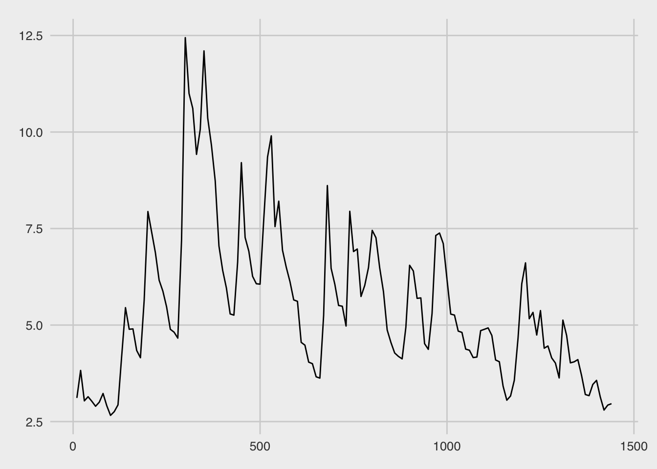
# Create model specification object (for priors, starting values, and proposal
# variances)
model_spec <- pulse_spec(location_prior_type = "order-statistic")

# Fit model (takes roughly 3-10 minutes)
#   Note: fit_pulse accepts a plain dataset with the time and concentration
#         variable names specified, or an object created by simulate_pulse()
fit_test   <- fit_pulse(.data = this_pulse,
                        iters = 250000,
                        thin = 50,
                        spec = model_spec,
                        verbose = FALSE)
# Inspect posterior chains
str(fit_test, max.level = 1)
## List of 7
## $ model : chr "single-subject"
## $ call : language fit_pulse(.data = this_pulse, spec = model_spec, iters = 250000, thin = 50, verbose = FALSE)
## $ common_chain:Classes 'tbl_df', 'tbl' and 'data.frame': 4500 obs. of 9 variables:
## $ pulse_chain :Classes 'tbl_df', 'tbl' and 'data.frame': 62661 obs. of 8 variables:
## $ data :List of 3
## ..- attr(*, "class")= chr "pulse_sim"
## $ options :List of 4
## $ spec :List of 4
## ..- attr(*, "class")= chr "pulse_spec"
## - attr(*, "class")= chr "pulse_fit"
common_chain(fit_test)
## # A tibble: 4,500 x 9
## iteration num_pulses baseline mean_pulse_mass mean_pulse_width halflife
## <int> <int> <dbl> <dbl> <dbl> <dbl>
## 1 25001 14 3.12 3.56 26.6 45.1
## 2 25051 13 3.12 3.70 27.3 47.2
## 3 25101 13 3.06 3.71 19.3 50.2
## 4 25151 14 3.11 3.36 13.4 49.0
## 5 25201 13 3.18 3.89 6.08 45.0
## 6 25251 13 3.10 3.11 1.85 53.9
## 7 25301 14 2.90 3.47 15.8 58.6
## 8 25351 12 3.01 4.59 29.1 56.0
## 9 25401 13 2.81 3.80 17.7 59.2
## 10 25451 13 3.12 3.62 22.2 51.3
## # ... with 4,490 more rows, and 3 more variables: model_error <dbl>,
## # sd_mass <dbl>, sd_widths <dbl>
pulse_chain(fit_test)
## # A tibble: 62,661 x 8
## iteration total_num_pulses pulse_num location mass width eta_mass
## <int> <int> <int> <dbl> <dbl> <dbl> <dbl>
## 1 25001 14 0 129 2.05 44.4 0.896
## 2 25001 14 1 189 4.62 66.0 4.59
## 3 25001 14 2 291 6.17 35.1 0.504
## 4 25001 14 3 328 6.29 72.0 1.00
## 5 25001 14 4 440 4.65 43.1 2.00
## 6 25001 14 5 503 3.36 37.0 0.863
## 7 25001 14 6 521 2.56 5.19 0.158
## 8 25001 14 7 671 4.34 56.9 1.40
## 9 25001 14 8 735 3.58 32.8 1.63
## 10 25001 14 9 791 2.50 64.8 0.0270
## # ... with 62,651 more rows, and 1 more variable: eta_width <dbl># Review traceplot and posterior distributions
bp_trace(fit_test)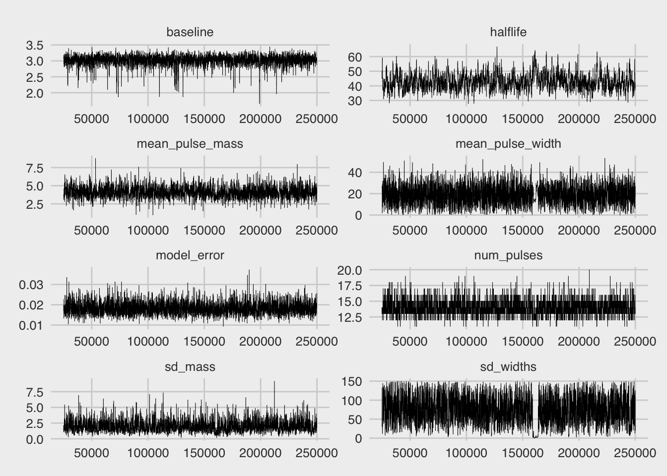
bp_posteriors(fit_test)
## Warning in if (type == "histogram") {: the condition has length > 1 and
## only the first element will be used
## `stat_bin()` using `bins = 30`. Pick better value with `binwidth`.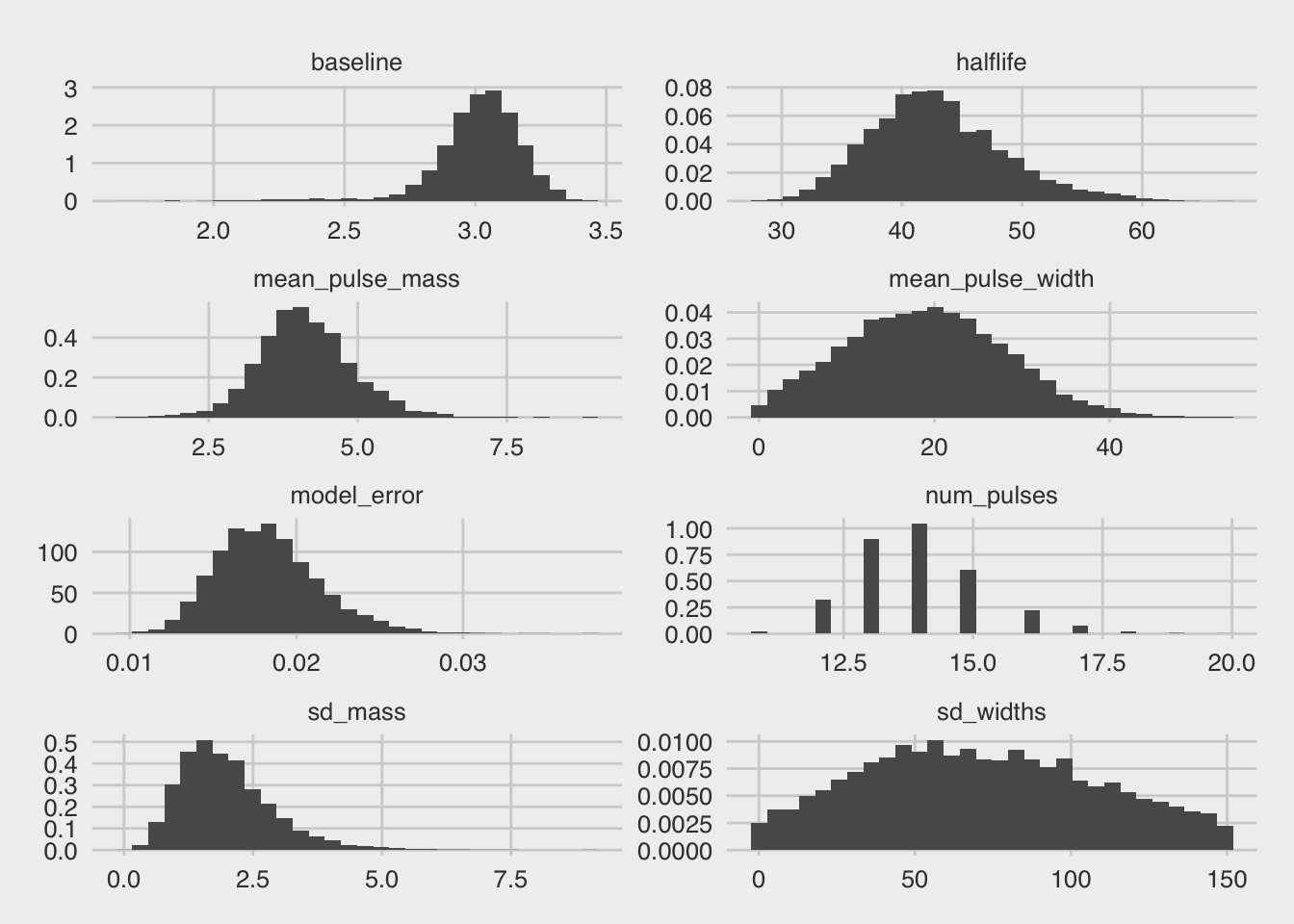
bp_location_posterior(fit_test)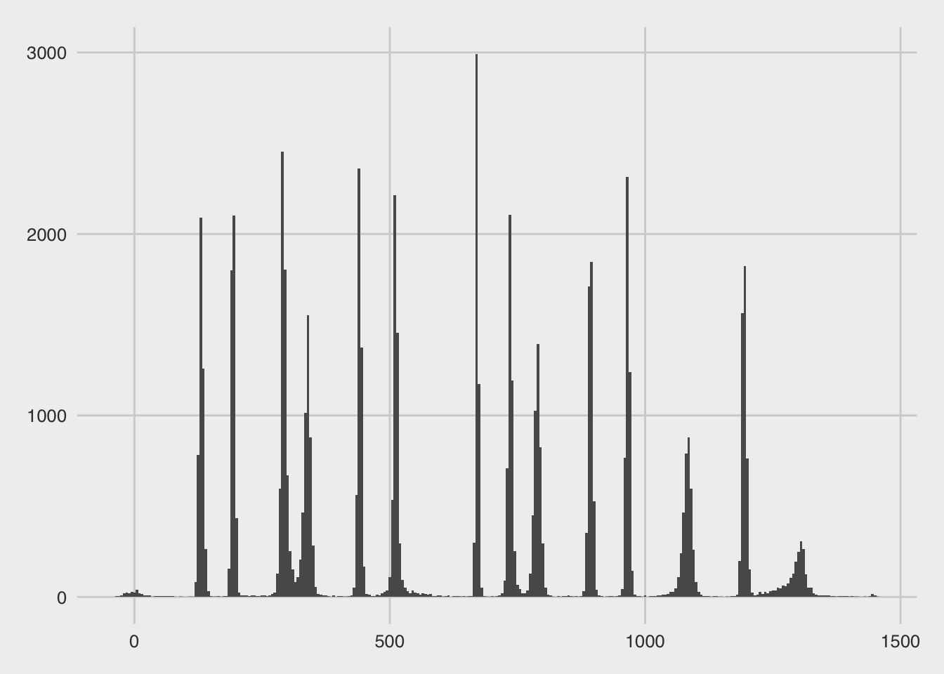
# Calculate mean and 80% HPD credible interval
rbind(
      common_chain(fit_test) %>%
        summarise_at(vars(num_pulses:sd_widths), mean),
      common_chain(fit_test) %>%
        select(-iteration) %>%
        as.mcmc %>%
        HPDinterval(., prob = 0.8) %>% t
      ) %>%
mutate(stat = c("mean", "lower", "upper")) %>%
gather(key = parameter, value = value, -stat) %>%
spread(key = stat, value = value)
## # A tibble: 8 x 4
##   parameter          lower    mean    upper
##   <chr>              <dbl>   <dbl>    <dbl>
## 1 baseline          2.86    3.01     3.21
## 2 halflife         35.5    42.9     49.4
## 3 mean_pulse_mass   3.06    4.13     4.98
## 4 mean_pulse_width  6.85   19.0     30.5
## 5 model_error       0.0140  0.0183   0.0216
## 6 num_pulses       12.0    13.9     15.0
## 7 sd_mass           0.838   1.98     2.92
## 8 sd_widths        19.5    71.3    120